Chaotic Dynamical System Maps as Optimization Problems

A few years ago I came across a paper that demonstrated a technique to estimate the value of parameters in dynamical systems–such as the gravitational constant acting on a double pendulum–to a precision some 13 orders of magnitude better than traditional approaches (A Global Approach to Parameter Estimation of Chaotic Dynamical Systems, Saipas 1992). This methodology has stuck with me as I begin to research Complex Systems, so I figured I’d look a little deeper and play around with this technique.

Description of the paper

To start, let’s show how the algorithm works. We define a complex dynamical system as:

(1) $\begin{equation*} z_{t+1} = z_t ^ {2} + c\end{equation*}$

where $z_t$ and c are complex numbers. This can be decomposed into the real-valued equations:

(2) $\begin{equation*} x_{t+1} = x_t ^ {2} - y_t^{2} + \lambda\end{equation*}$

(3) $\begin{equation*} y_{t+1} = 2 x_t y_t + \epsilon\end{equation*}$

We run this system until it escapes a given radius $R_{max}$ (i.e. $\lVert z_t \rVert > R_{max}$ , or $\sqrt{x_t^2 + y_t^2} > R_{max}$ ), or until we’ve reached a maximum timestep $T_max$ , and record the final timestep t in which the system terminated. For these experiments, we set $T_{max}$ = 1000 and $R_{max}$ = 100.

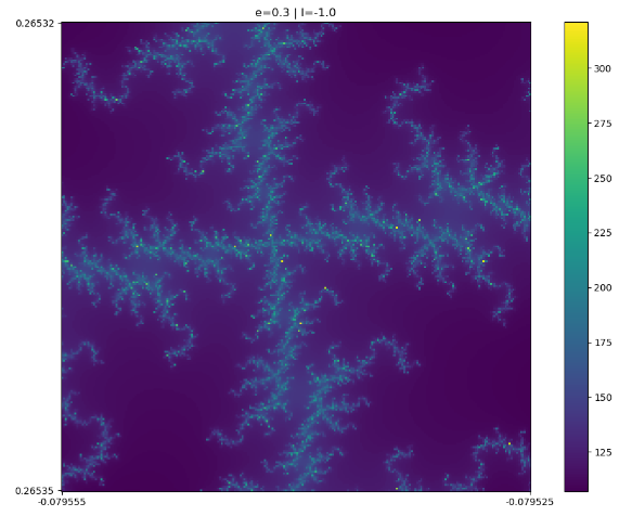
Ok, let’s look at the behavior this system produces. If we set $\lambda$ = -1.0 and $\epsilon$ = 0.30, and run this system for an array of starting values (x,y) in [(0.079555, -0.079525], [0.2653120, 0.265350]), we get the following image:

Figure 1: Values of t generated in a small window.

Pretty cool, right? We can also increase the contrast in this image by applying a modulo filter–calculating the remainder when dividing each pixel in the image by a fixed number: $t -> t % n, also written as t -> Remainder(t/n)$ , where n is an integer.
Here’s what the image looks like if we apply a modulo filter with n=10:

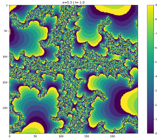
Figure 2: Values of (t % 10) generated in a small window

Interestingly, because this is a complex system, if we change any parameter (including $\lambda or \epsilon$ ) by a small amount, the dynamics of the system change considerably. We can clearly see this if we look at these same images, but with $\lambda = -1.00001$ :

Figure 3: The simulation as re-run for a small change in Lambda

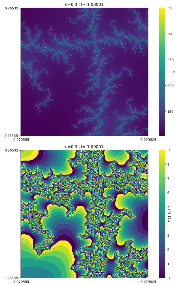
That’s a reasonably large difference in image for a parameter change of 10E-5.

Saipas takes this one step further by demonstrating experimentally that the difference between two images has a local minima that is unimodal with very nice properties, and that a simple optimizer (the Golden Section Method) is able to find the local minima with very high accuracy. Check out the paper for more details.

Nonlocal Estimation

I became curious about the bounds in which this algorithm is unimodal: under what conditions do more local optima appear?
So, I built a visualization that shows the value of this error function for 21 points evenly sampled from a [+3, …. -3] range around the true value, samp. It turns out that the error function has one clear local minima, and that the global optimum is not so easy to find after all–from values of 0.5 onwards, local search algorithms would find a local minima.

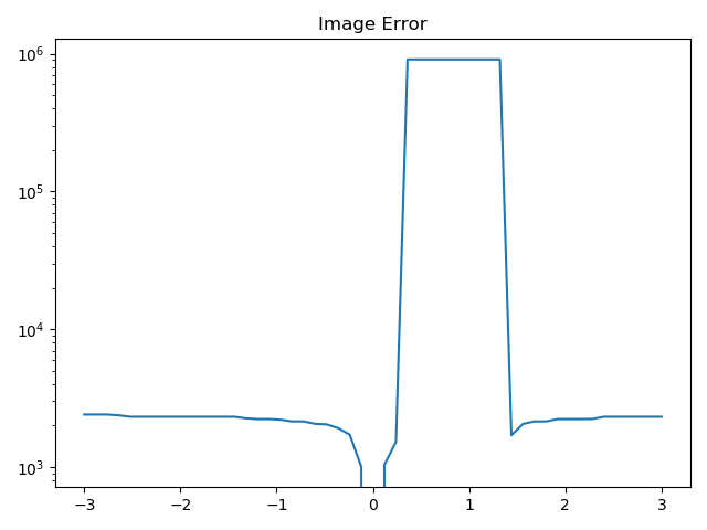
$Image Error vs \delta\lambda. The optimum value is found at \delta\lambda=0.$

Looking at this same problem, but from the perspective of the MODULO image makes the problem even harder. As the modulo decreases (i.e. as we see fewer ‘contours’ in the image), the error function has more local minima and has higher local variability.

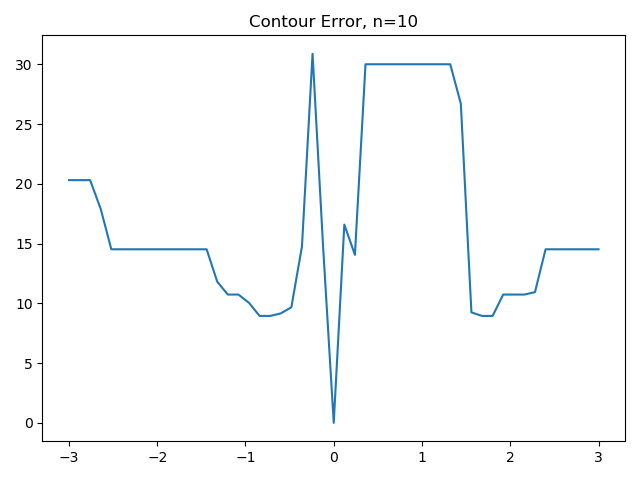
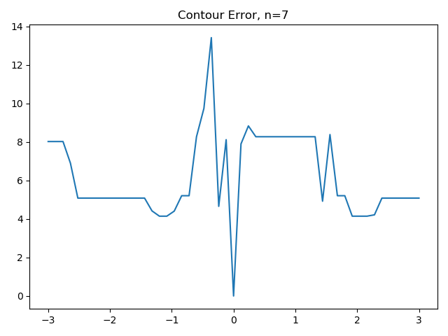
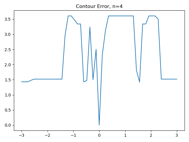
As a result, this problem has a tunable level of difficulty, measured in terms of the number of local minima per unit parameter distance. The problem also has a known value for the global minima (i.e. error = 0), which makes it an interesting choice for evaluating the general effectiveness of optimization algorithms that search a subspace for global minima, and try not to get stuck in local minima in the search process.

Next Steps

It would be interesting to see how the error function varies with a higher resolution, or how it varies as more parameters are changed (i.e. varying lambda and epsilon, and making a 2D graph of the error function).

It could also be interesting to see if these findings apply to general linear systems of the form:

(4) $\begin{equation*}X = \begin{bmatrix} x_1 \\ x_2 \end{bmatrix} \end{equation*}$

(5) $\begin{equation*}X_{n+1} = X_n * \begin{bmatrix} a_{11} & a_{12} \\ a_{21} & a_{22} \end{bmatrix} + \begin{bmatrix} b_1 \\ b_2 \end{bmatrix} \end{equation*}$

While these linear systems may display simpler properties, it would be possible to estimate each of the parameters $a_{n,m} and b_n$ , making the resulting optimization problem more difficult.

Finally, it could be interesting to evaluate the relative success of various search algorithms using this approach:

Genetic
Grid / Random
Simple Random Search
Particle Swarm Optimization
Emergent Optimization