Network Specialization

Neural networks have achieved great success over the last two decades in solving challenging problems, from diagnosing pneumonia in chest x-rays to playing a wide array of games like Starcraft and Chess. Despite recent advances, neural networks remain challenged at solving problems that contain multiple distinct sub-problems, such as an arithmetic problem set that contains both addition and division problems.

In this post, I first define an arithmetic dataset that contains addition, subtraction, multiplication, and division problems. Next, I show that despite the apparent simplicity of the problem, both wide and deep neural networks fail to reach near-zero training or testing error when training on this dataset. I then show that dividing the dataset into four sub-problems and training four networks (one on each sub-problem) reaches near-zero training and testing error with significantly smaller networks than the generalist one-network approach. This finding indicates that some problems are better solved not by larger ‘generalist’ networks that learn to fit all data, but by dividing the problem into sub-problems and training a set of networks that specialize in solving each sub-problem. Finally, I suggest three promising directions for future work that seek to find and train an optimal set of specialist networks for a given optimization problem.

The Problem + Dataset

Let’s study with a simple problem: Arithmetic! We want to teach a network to solve simple addition, subtraction, multiplication, and division problems, under a specific range. The function is thus:

(1)  

where x, y [-10, 10], the four functions possible are addition, subtraction, multiplication, and division:

   

The output z is constrained to be between -100 and 100 so that the division doesn’t blow up:

(2)  

We can specify each problem of this type as an array of three numbers: [x, y, n], where n is an integer describing the problem that needs to be solved: {0: x+y, 1: x-y, 2: x*y, 3: x/y}. So, a typical problem of this form could be: [1, 4, 0], with a correct answer of: 1+4=5.

I created a randomly-generated dataset of 500 training and 50 testing datapoints of this type by randomly sampling two floats (x,y) between (-10 ,10) and one integer (n) between [1, 4], and then calculating the corresponding target value (z) between (-100, 100). All of the following algorithms were evaluated using this same dataset.

Training a Typical Neural Network

The first approach I tried in solving this problem was to create a simple Neural Network (an MLPRegressor in sklearn with default parameters) and hand it all of the data I had on the problem.

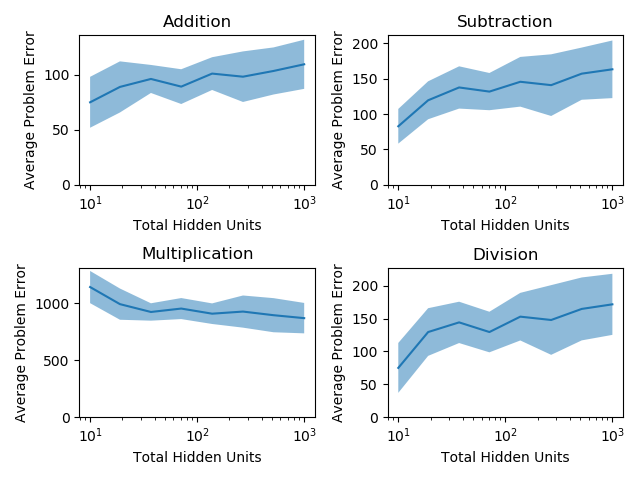
Below, I’ve plotted the network performance on this problem, subsegmented by subproblem type and measured using the Mean Squared Error on the testing data, by the number of hidden units used to solve the problem. In this example, the networks are shallow (1 hidden layer). The dark blue line in each graph represents the mean performance of 25 randomly initialized networks, and the shaded blue region represents 1 standard deviation of these 25 network performances.

There are two surprising findings from the graph above: first, increasing the width of the hidden layer here doesn’t meaningfully increase the accuracy of the network. Generally, we expect bigger networks with more hidden units to perform better, because they’re able to fit more complex functions in the training data. Second, the networks didn’t seem to accurately solve ANY of the sub-problems: it seems that the presence of all four sub-problems made it hard to even solve one sub-problem accurately.

One Network Per Subproblem

Clearly this problem is solvable with 0 error, and a traditional network architecture isn’t achieving the kinds of error rates we want, so how could we design a fix for this problem?

Since we understand the problem deeply–it’s composed of four sub-problems that require very different solutions to one another for a given (x,y) pair–we can design an architecture that splits the data into subproblems, and then trains each sub-network to solve a different one. Specifically, we’ll split the training / testing data into four sets of training / testing data (with average size 1/4 of the original dataset), one for each problem type. Then, we’ll train each of four new neural networks (with 1/4 the original network’s width) on one of the new datasets. In essence, we’ll have created one network that specializes in addition problems, one that specializes in subtraction, etc.

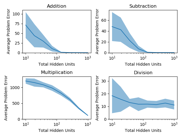
Importantly, with this design we can effectively and fairly compare the new subproblem architecture with the original one-shot architecture, because both architectures train and test on the same amount of total data using the same resources. The subproblem architecture’s performance on each subproblem is shown below:

Amazingly, with this decomposition into sub-networks, each problem becomes easily solvable: the networks produce nearly-correct outputs on each subproblem while using the same computational resources and same data! Also as a result of this change, making the network more complex with more hidden units now increases the network accuracy on each problem. In summary, by dividing the problem into parts, we’ve made the problem tractable for a typical network, not only reducing the computational overhead to reach a reasonable answer but also significantly increasing the network’s accuracy.

Why?

Why do we observe this effect: that problems become tractable when decomposed into sub-problems?

I suspect that the reason lies with the mechanics of backpropagation and gradient descent: typical neural network architectures backpropagate the error from all datapoints through to each hidden unit in the network–meaning that each hidden unit is optimized to be a generalist: good at providing input to a wide range of problems. No hidden unit is able to be a specialist, and dedicate themselves to one specific problem type.

By breaking the network up into four discrete sub-networks, and training each set of hidden units in each sub-network only on the datapoints associated with a single sub-problem, we instead ask each hidden unit to be a specialist in one problem type only. This makes the overall problem that each hidden unit faces much simpler, and ultimately enables the network as a whole to perform better.

Next Steps

We know that hard problems, especially those composed of multiple sub-problems, require a different approach to learning than the typical shotgun approach used by single neural network architectures. In short, nodes in the network need to be able to specialize in problem types in order to solve these problems. The question is, how can we enable this specialization to spontaneously emerge based on the problem at hand?

Ideally, we want an algorithm that adapts to the problem at hand: specializing to the degree that the problem requires it. In fact, this could be equally viewed as a challenge in identifying the structure of the problem at hand, since a knowledge of the problem structure lends itself directly to an applied solution.

The development of such an algorithm could take the form of: (i) an error-clustering algorithm that locates clusters of datapoints with similar error profiles and creates sub-networks to specialize in these cases, (ii) an emergent network algorithm, like one that I wrote about here, where nodes explore connecting to other nodes in order to maximize their predictive utility, or (iii) an evolutionary algorithm that selectively propagates the fittest data partitions. I hope to write a post soon on these promising algorithms.

[Update 10/6/20]

As it turns out, deeper neural networks — of depth 5 and greater — do fit this Arithmetic problem with reasonable accuracy, even with relatively few hidden units. It appears that reducing the number of problems the network is trying to fit at once has the effect of reducing the total number of hidden units needed to achieve a high level of accuracy. This makes sense, because by segregating the data by problem type, we’re building into the network some information about the problem itself.

There still may be opportunities to use this effect to reduce the compute requirements of modern neural networks–for example, in learning this segregation pattern from new data.

Appendix: Notes

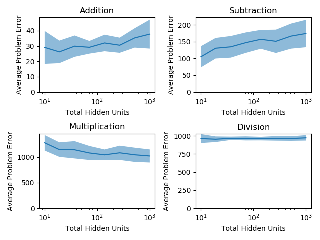
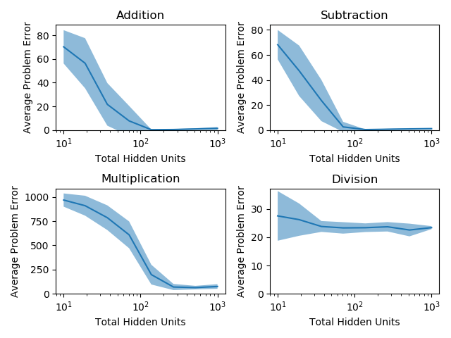
This paradigm appears to hold for deeper networks as well: if we use a depth 2 network, where the first layer remains the same width as previously and the second layer is half the width of the first, we get the following performance from the single network and sub-network cases: